PowerPivot: Excel PivotTables on Steroids?

Pivot tables in Excel are an excellent tool and are used by many to aggregate and summarise data for reporting purposes. For example: A pivot table could be used to display product sales by month vs. region, department vs. year or as shown below: product vs. discount type:

If the original data is available in an Excel worksheet then the “Insert > Pivot Table” menu inserts a pivot table into the worksheet and presents a field list that can be used to drag and drop the required fields onto the table. This is all very straightforward and very powerful.

Earlier versions of Excel were limited to 65535 rows a worksheet. Later versions increased the limit to 1048576 rows. However the processing involved in combining data from worksheets and pivoting is computationally expensive and pivoting large volumes of data quickly becomes too slow. For data sets in excess of a million of rows it is simply not possible.

Excel pivot tables can also connect directly to external data sources such as SQL Server databases and cubes in SQL Server Analysis Server. Using an external data source in this way, and cubes in particular, is the usual way to pivot large volumes of data. Coverage of Analysis Server and the creation of cubes are beyond the scope of the blog, but they are a kind of large scale pivot table based on raw data in a database.

The snag is that although Excel pivot tables can be setup and used by a power user, Analysis Server cubes require a developer. Until that is, PowerPivot came on the scene with the release of SQL Server 2008 R2 and SQL Server 2012. PowerPivot allows a power user to combine data from Excel and external data sources such as databases and create large scale pivot tables without a developer. PowerPivot is essentially a cut down version of Analysis Server that is built into Excel. There is also a SharePoint version as well.

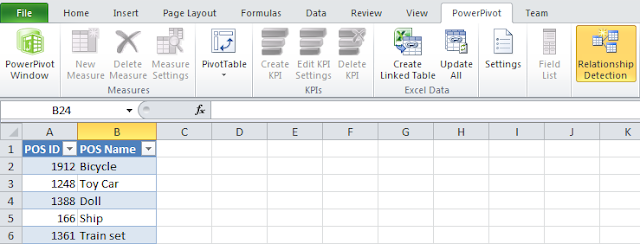
To trial the capabilities of PowerPivot I selected a customer database containing a table with 3.6 million rows of product sales and discount information. The database did not contain user friendly names for either the products or the discounts and so this information was added as Excel worksheets. I then selected the “Create Linked Table” on the “PowerPivot” menu as shown below to link my product and discount worksheets to PowerPivot (as shown below):

The next step was to select the “PowerPivot Window” menu in Excel followed by the “From Database” menu to create a sales data set base on a SQL query as shown below (as an alternative whole database tables can be loaded, avoiding the need to write SQL): 

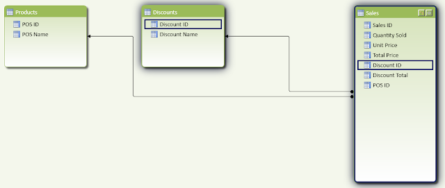
Next the “Diagram View” was used to join the SQL database to the two linked worksheets by dragging and dropping the keys:

At this point there is data from 3.6 million rows linked to two worksheets all in PowerPivot. New calculated columns can be added just by entering a normal Excel formula, as shown below for the new column CalculatedColumn1.

In the “Calculation Area” (the lower half of the screen below the data) new aggregate calculations such as “=Min([Total Price])”, can be added, again by just using standard Excel formulas. However PowerPivot automatically calculates all the obvious ones and so there is no need create simple examples like this.

Once the data is in place, click the “PivotTable” menu to create pivot tables and charts from the data in the normal Excel way, but this time using millions of rows of data.

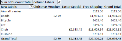
I opted to select “POS Name” and “Discount Name” as slicers to allow the user to easily select the required data with the mouse. The pivot table shows discount and total price for the selected products and discounts. The pivot chart shows the breakdown of the discounts for the selected products and discounts. Selecting any combination of products and discounts in the slicers on the left recalculates and redisplays the table and chart in a fraction of section, even with 3.6 million rows, and I could go way higher than this.

Essentially this example shows how easy it is to create large scale pivot tables in Excel without having to manually define and create cubes using Analysis Server.

This article is based on SQL Server 2012 PowerPivot for Excel in Excel 2010.